How ELT Schedules Can Improve Root Cause Analysis For Data Engineers
“Correlation doesn’t imply causation, but it does waggle its eyebrows suggestively and gesture furtively while mouthing ‘look over there’” – Randall Munroe
In this article, Ryan Kearns, co-author of O’Reilly’s Data Quality Fundamentals and a data scientist at Monte Carlo, discusses the limitations of segmentation analysis when it comes to root cause analysis for data teams, and proposes a better approach: ELT schedules as Bayesian Networks.
Data engineering and root cause analysis
“Root Cause Analysis” (RCA), a procedure for defining the fundamental explanation of an issue, is a bit of a sanctified term in the software world.
Ongoing issues don’t really end until the root cause is established. Whether you’re dealing with a broken API call, a website that’s not loading, or a metric that’s gone awry, identifying the root cause is always fundamental in the resolution process. At that point, engineers can explain the source of the failure, work towards shipping a fix, and mitigate the issue in the future.
In the new field of data observability, RCA is equally essential. The fastest way to make bad data good is to understand why it went bad in the first place. After all, once we detect the data is bad, the first thing we want to know is why.
Why are 10% of the rows suddenly filled with NULL values in your all-important marketing spend table? Why is the customer_uuid field suddenly showing tons of duplicates when it is supposed to be unique?
However, we data professionals are starting to use “RCA” to refer to tools that assist in RCA workflows, not tools that do any actual RCA themselves. This may sound trivial but the difference is significant. For example, many data quality RCA approaches use segmentation analysis: identifying responsible segments of the data that give better context to the incident.
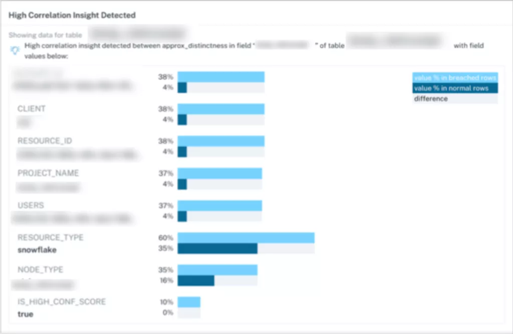
Segmentation analysis is an excellent correlative feature to give greater context to a data incident. Often, segmentation analysis may point you towards the root cause of an issue.
This can occur when:
- The on-call engineer has lots of context about the table in question.
- The segmentation analysis is sparse – that is, it returns only select correlations that a human could reasonably parse.
- The segmentation analysis is meaningful – that is, the correlations returned make actual sense and tell a story.
In the above case, upstream changes in an ELT job on several customers’ data sources caused an important metric for our machine learning models to drift significantly from the baseline. Segmentation analysis allowed us to attribute the drift to that specific upstream change.
Notice that there’s nothing in the segmentation analysis itself that identifies the root cause – an engineer with knowledge of the change was on-scene to connect the dots. Specifically here, note that one RESOURCE_ID figures in 4% of all records, but in 38% of the records with anomalous importance_scores. Turns out, this problem occurred with just three customers with the same edge-case integration setup, so we could quickly roll back the recent change to those environments.
Where correlation breaks down
But let’s think about a slightly different problem. What if, instead of just an ELT change for these three customers, we had a failure affecting the whole ELT pipeline?
If a table fails to update, one bad SQL LEFT JOIN could result in dozens of downstream columns turning NULL all at the same time. If everything in the downstream table has caught fire, segmentation analysis won’t do anything to help us.
We might see hundreds of notifications like “Field X is 100% correlated with field Y!” – and maybe one of these correlations hints at the actual root cause. More likely than not, you’ll be dealing with countless comorbidities of the same upstream symptom.
There’s a deeper point about what’s missing here, though. Segmentation analysis assumes that just looking at one table constitutes sufficient RCA. In any modern cloud data infrastructure, though, no table ever stands alone.
Tables rarely contain the root causes of their own data downtime. ELT pipelines time out, schemas are unwittingly changed, API functionality deprecates. We have seen this reality in our own data about data observability. We find that our “High Correlation Insights” feature only applies to ~4.4% of the anomalies we catch.
Data quality issues happen in context, and we rely on data engineers to know that context.
With approaches like segmentation analysis, we shift very little of that burden to the RCA tools themselves, even when we could be doing so, saving ourselves time and headaches in the process.
Here’s why data engineering teams need to go beyond segmentation analysis when it comes to reducing time to resolution for data downtime.
Case study: in-context RCA for data downtime
It’s time we take RCA for data downtime seriously, which means taking the structure of data downtime seriously.
Modern data pipelines are complicated, interdependent systems with upstream and downstream dependencies. This includes software, data, and schedule dependencies, in other words, lineage.
When data goes wrong, something upstream in the pipeline – software, data, or schedule – has to be wrong, too. When dealing with vexing, real-time issues with data, we often forget that data environments are highly structured. When it comes to conducting RCA on broken data systems, we can – and should – use this to our advantage.
To make my point concrete, let’s look at one specific mainstay in the modern data pipeline: ELT jobs. ELT platforms, like dbt, run data transformations using scheduled DAGs – Directed Acyclic Graphs.
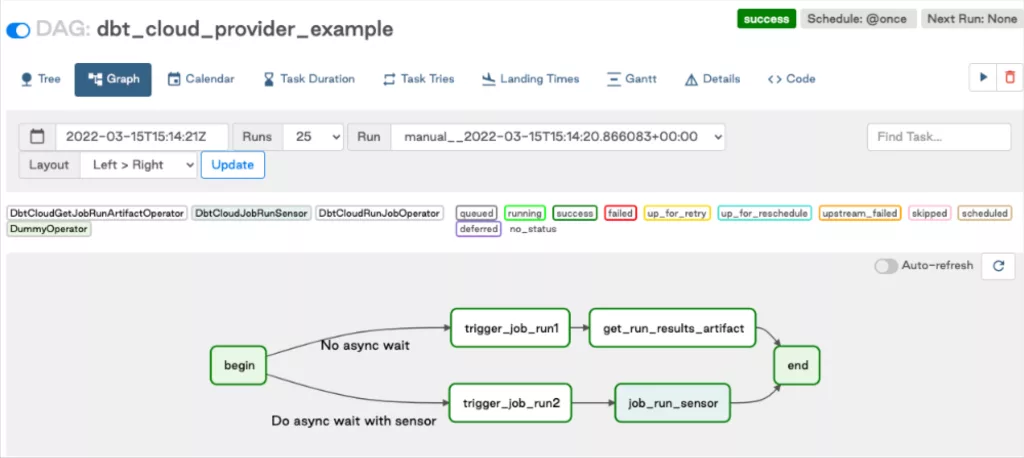
DAGs are not arbitrary mathematical structures. They exhibit plenty of neat properties (transitive closure, topological ordering, etc.) that dramatically reduce the complexity of many graph algorithm problems (like finding shortest paths).
They’re also the structure of Bayesian networks, powerful computational devices that we can use for (real) data downtime RCA. In fact, the structure of Bayesian networks modeling ELT schedules is simpler than a generic Bayesian network! Let’s walk through this via an example.
An example DAG
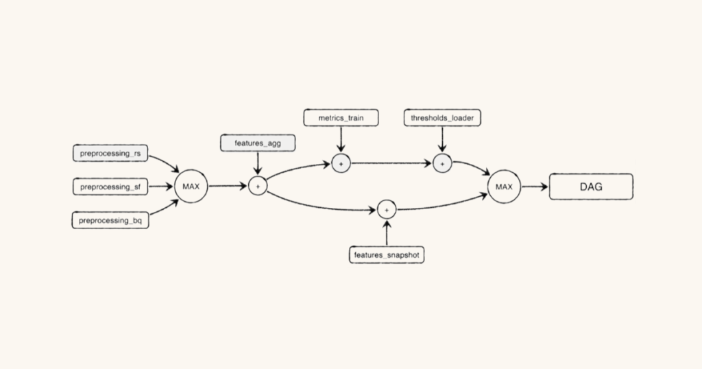
Let’s model a simple data downtime problem to show how. Here’s a simplified DAG showcasing part of an ELT schedule that runs at Monte Carlo:

This job combines some feature aggregation steps with a model training step, followed by some export steps. It’s a part of a larger machine learning pipeline. Note that _rs, _sf, and _bq refer to preprocessing metrics collected from Redshift, Snowflake, and BigQuery environments respectively.
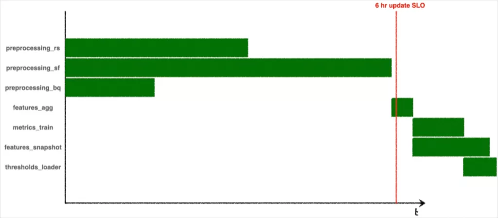
Here’s the corresponding Gantt chart from one run:
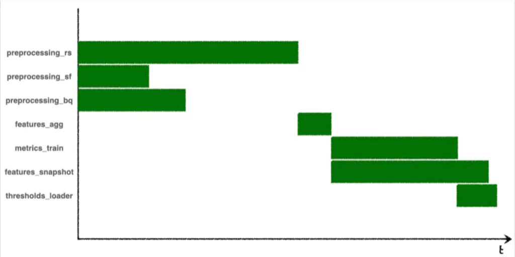
Notice anything structurally interesting?
features_aggcan’t run until all of thepreprocessing_steps are complete, because those preprocessing steps are upstream dependencies in the DAG. Even thoughpreprocessing_sffinished early on this run, progress in the DAG is bottlenecked untilpreprocessing_rsfinishes.
features_snapshottakes longer to run thanmetrics_train, but it doesn’t bottleneck the start ofthresholds_loader, because it’s not an upstream dependency.
Calculating the DAG’s runtime
Oftentimes, data engineers want to predict the runtime of the entire DAG, whether to set an SLA or be assured that metrics will update with a certain cadence. If we want to know how long the whole DAG takes to run, we can’t just sum up all the individual job runtimes. We can’t take the maximum runtime either. Instead, we have to resort to features of the DAG. Which jobs are upstream from which other ones? Which jobs are the bottlenecks?
In this case, the runtime will always be given as this function of job runtimes:
time(DAG) = MAX(time(preprocessing_rs),
     time(preprocessing_sf),
     time(preprocessing_bq)) +
 time(features_agg) +
 MAX(time(features_snapshot),
     time(metrics_train) + time(thresholds_loader))
Maybe this equation is daunting, but the rules for creating it are simple:
- If processes happen in parallel, take the MAX() of their runtimes
- If processes happen in sequence (or in “series”), take the sum of their runtimes
With these two rules together, you can take any ELT DAG and build an equation that calculates its total runtime.
Using schedule dependencies to solve data freshness anomalies
All well and good when the DAG finishes on time. Of course, the interesting case is when it doesn’t.
Many teams define SLOs to guarantee that certain processes complete by certain times. This particular DAG in our system runs every 6 hours. Sometimes, it fails or stalls, and in some cases data (from thresholds_loader) won’t arrive for 7 or 8 hours. In these cases we’d like to understand the root cause – why is our DAG not performing as expected? And what do we need to change to keep the updates coming on schedule?
Concretely, a Gantt chart for an SLO-breaching DAG run could look like this:
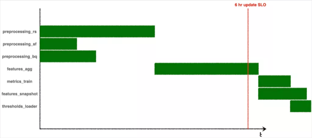
Or it could look like this:
How do we say, mathematically, which jobs fault it was that the DAG took too long?
Enter Bayesian networks. Once again, we’ll turn to the ELT DAG. We already gave the equation for time(DAG) above, which tells us the total runtime as a function of job runtimes. If we know the runtimes from a particular DAG run we’re interested in, this is great. But what about in general? How long should we expect the DAG to take, probabilistically?
To think probabilistically we should turn to Bayesian networks, which means we need to make a new DAG… out of our DAG. (Don’t panic! Bayesian networks are just types of DAGs too – special ones intended to answer probabilistic queries using statistics and causal inference.)
To turn our ELT DAG into a Bayesian network we need to think of each job runtime no longer as a discrete value (like, “43 seconds”), but instead as a variable drawn from a distribution of runtimes.
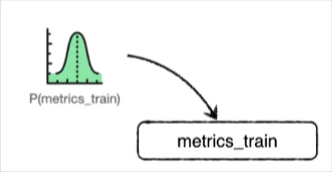
Computational processes – especially ones that deal with data – often take a sort of consistent time to complete, but there will be variance. Maybe your load balancer is having a bad day, or maybe someone’s just barraged your API with requests. Maybe one of Redshift, Snowflake, or BigQuery is having independent performance issues.
So let’s start by making all the runtimes probabilistic. Now, each node elt_job represents a random variable, where P(elt_job < t) represents the probability that that job finishes in less than t seconds.

Ok… so this is our Bayesian network? Doesn’t it look exactly the same as the ELT DAG we had earlier?
Well, this is a legitimate Bayesian network, but it’s not a proper representation of our DAG at all. Why? We’ve actually thrown out some super valuable information – namely, the two rules about runtimes we discovered earlier. Here they are again:
- If processes happen in parallel, take the MAX() of their runtimes
- If processes happen in sequence (or in “series”), take the sum of their runtimes
Can we account for these rules in our Bayesian network? Spoiler alert: we can, and it decreases the complexity of our network dramatically. To do so we need to invent two “special” kinds of nodes with simple probability distributions. First, for parallel processes, we’ll have a “MAX” node, with a probability distribution given by:

For sequential processes, we’ll also have a “+” node, with a probability distribution given by:

Is this overly academically pedantic? Yes. Are we stretching the definition of a “random” variable? Maybe. But it’s really the lack of randomness here that’s important to take away, since it makes the resulting Bayesian network so much simpler computationally.
Here’s a transformed Bayesian network using those two special nodes we just defined:

The final node, DAG, is a random variable whose value depends entirely on the probabilistic runtimes of all the jobs (e.g. the variables features_agg, metrics_train, etc.) together with all the summing and maxing. More precisely, we know that:
P(DAG) = MAX(P(preprocessing_rs),
  P(preprocessing_sf),
  P(preprocessing_bq)) +
   P(features_agg) +
   MAX(P(features_snapshot),
       P(metrics_train) + P(thresholds_loader))
This equation looks a lot like the equation for the discrete runtime case, except that the discrete runtimes (time) have been replaced with probabilities for each runtime (P). The summing and maxing remained the same, though, which makes this equation pretty tractable.
Of course, the distributions like P(preprocessing_rs) aren’t going to magically fall out of the sky at this point. You’ll have to estimate these from a finite number of runs of the DAG itself. There’s a whole rabbit hole to fall into here, too, but for now let’s assume you can fit normal distributions to the runtime of each job in the ELT DAG.
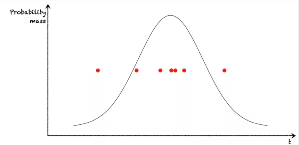
So now let’s get concrete. We can see that a lot of questions we’d like to ask about the DAG can be formulated as queries against our new Bayesian network.
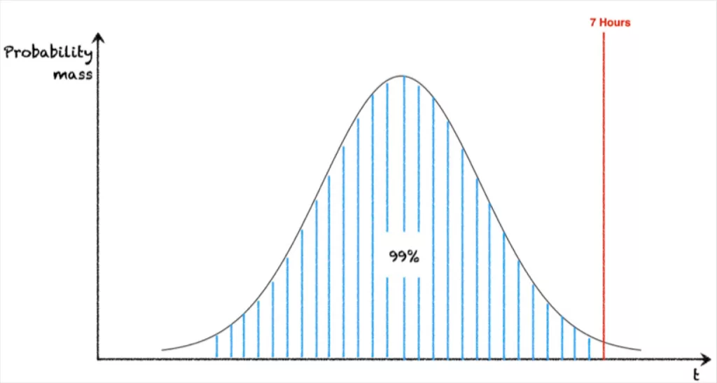
Q: The DAG just took 7 hours to run. Is that abnormal?
A: What’s the value of P(DAG < 7 hours)? If that number is “high” – let’s say it’s 99% – then yeah! Abnormal! A 7 hour DAG runtime is a 1% likely occurrence.
Q: Did the features_snapshot job take too long to run?
A: Say the features_snapshot job ran in time t. What’s P(features_snapshot < t)? If this number is “high” – let’s say it’s 80% – then yes! t is a pretty abnormal runtime.
Q: (THE RCA QUESTION): Was features_snapshot responsible for the DAG taking 7 hours to run? To what extent?
A: What’s P(DAG < 7 | features_snapshot = t)? If this number is high, then it’s quite likely that the DAG can finish in under 7 hours even with features_snapshot taking t seconds. If it’s low, then it seems more likely that the DAG was bottlenecked by this one job. It’s even more likely if P(DAG < 7 hours) and P(features_snapshot >= t) are low. It’s especially likely if
P(DAG < 7 | features_snapshot = E[features_snapshot])
is high, which says that the DAG would have likely finished in fewer than 7 hours if features_snapshot had taken the expected amount of time.
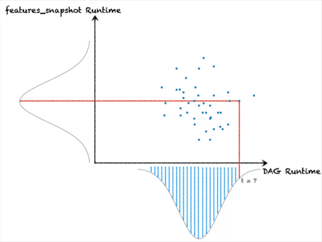
As we can see, the causal tapestry to explore here is rich, even without venturing into causal inference for field-level anomalies, such as an unexpected uptick in NULL-rate or a sharp decrease in some key metric. What’s more, Bayesian networks and causal inference allow us to pose questions about actual RCA with math, rather than surfacing correlative hints that a human engineer has to stitch together into a narrative.
In my opinion, domains like these are the real forefront of RCA for data quality issues: leaning into the unique structure of data infrastructure, leveraging lineage, and treating software, data, and scheduling dependencies as the first-class citizens of causal inference for data.
Data teams have the potential to automate and scale much of the root cause analysis for data downtime, and segmentation analysis on a per-table basis is not going to get us there.
Until then, here’s wishing you no data downtime!
What do you think? Reach out to Ryan Kearns to share your thoughts. And if data quality through faster, more streamlined incident resolution and lineage is top of mind for your organization this year, schedule a demo with our team.
Our promise: we will show you the product.
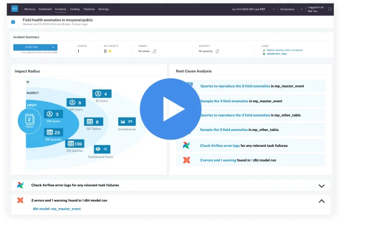 Product demo.
 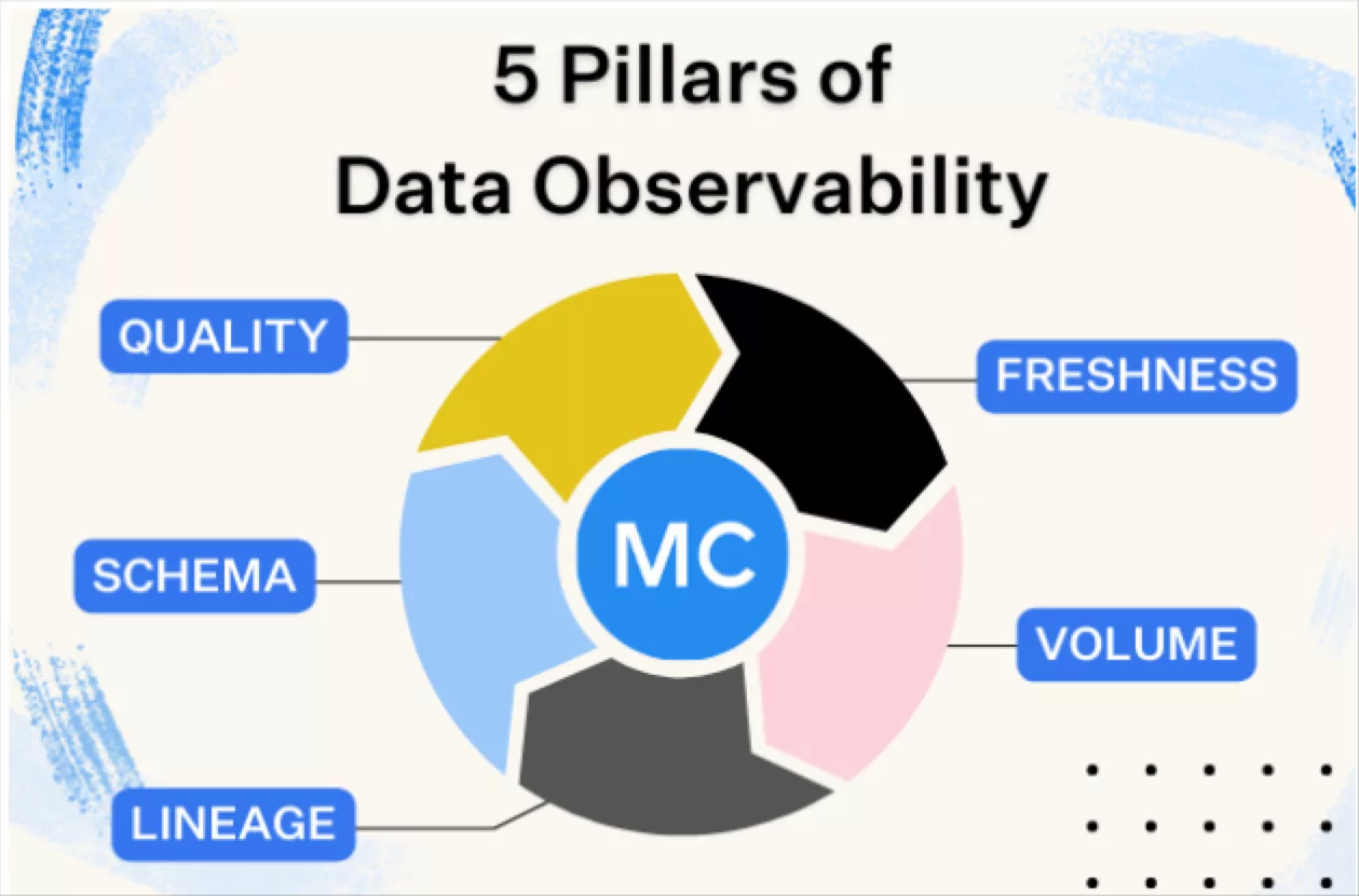 What is data observability?
 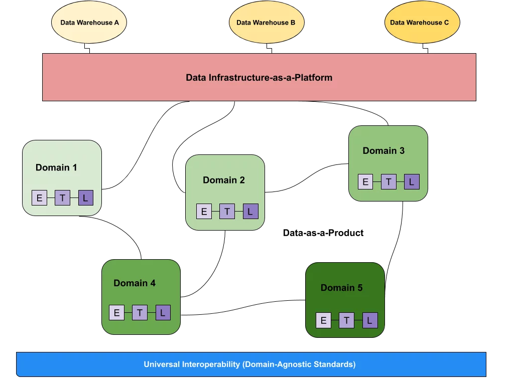 What is a data mesh--and how not to mesh it up
  The ULTIMATE Guide To Data Lineage
